![]()

The Chi-Square Test
What is Chi-Square?
As is already clear from the Binomial Experiment (Mayo, ch. 5, Figure 5.2), any statistical test comes down to calculating the probability that a certain result holds according to the null hypothesis. A convenient and much used method for this purpose is the chi(°ď)-square test, first proposed by Karl Pearson; and this is very useful especially when the experimental results are classified into several groups (which are mutually exclusive). Since Mayo does not say anything about this, let me add this note.
Karl Pearson (1857-1936)
As an example, take Mendel's famous experiment with peas (the materials are drawn from Harald Cramer, The Elements of Probability Theory, Wiley, 1955, 219). With this example, you can get an idea of what chi-square is, and how chi-square test goes. In one of his experiment, Mendel obtained 556 peas, classified according to shape (either Roud or angular) and color (either Yellow or green); Round and Yellow are dominant, the capital letters signifying a dominant gene. Thus according to Mendel's law, the following 16 genotypes have an equal probability (our students should be familiar with this logical pattern!).
RRYY, RRYg, RRgY, RRgg, RaYY, RaYg, RagY, Ragg,
aRYY, aRYg, aRgY, aRgg, aaYY, aaYg, aagY, aagg.
However, since phenotypes are governed by dominant genes, we should expect the following proportion for the four types:
- Round and Yellow: 9/16
- Round and green: 3/16
- angular and Yellow: 3/16
- angular and green: 1/16
Now, Mendel obtained the following data by his experiment:
Ş@ Ş@
All right. How should we check whether or not these data fit the Mendel's expectation (hypothesis)? Here the chi-square works well. Let us define a quantity called the chi-square (°ď°ď) as follows. (1) First, take the square of each difference, and divide it by the expected frequency; then (2) take the sum of all. This is the chi-square of these data. In short, the chi-square is a sum of each weighted (squared) difference. We take the square because we wish to treat all differences (positive as well as negative) on a par.
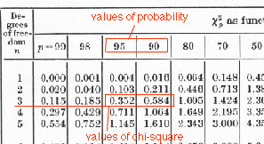
Since we have 4 groups, and since if 3 groups are given then everything can be determined, we say this distribution has "3 degrees of freedom". And for our data, the value of chi-square is:
°ď°ď = 5.0625/312.75 + 14.0625/104.25 + 10.5625/104.25 + 7.5625/34.75
= 0.016 + 0.135 + 0.101 + 0.218 = 0.470
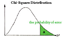
Now this value is useful in that we can obtain the probability that the data occurs (and the probability that the data are an error, as well; see the figure of chi-square distribution), from this value; in any standard textbook of statistics, you can find a table of chi-square distribution, and from this table you can obtain that probability. In our case, the probability falls between 0.90 and 0.95 (see the partial table), since 0.470 comes in between 0.352 and 0.584 in the table. That is, given Mendel's hypothesis, it is quite likely that we obtain these data (distribution). Thus on the customary standard of significance level, it may be judged that this hypothesis passed the test. See the graph of the chi-square (with the degree of freedom 3), and its relation to the probability of an error; to the extent this probability is small, the test is severe.
[This is the curve for the degree of freedom 3]
Table of chi-square distribution; look at the line of degree 3
Readers who need more explanation should consult Ishikawa (1997), ch. 4, pp.63-71. There, a similar problem (in terms of dice) is treated more in detail. Try to calculate probabilities yourself (on a computer)!ĆëĆÉÓĆlŞw°T°C°R°ŮŽExcelÎíÉŤáă˙ÔvĹÝĆęŞxŃŰ÷¤śoäŞA1997ŞB
INDEX- CV- PUBLS.- PICT.ESSAYS- ABSTRACTS- INDEXŞELAPLACE- OL.ESSAYS-CRS.MATERIALS
Last modified Jan. 26, 2003. (c) Soshichi Uchii