![]()

Basics of Statistics
Mean, Deviation, Variance (Dispersion), and Standard Deviation
These are some of the essential concepts in mathematical statistics; without clear understanding of these, it may be rather hard to follow Mayo's arguments. However, unfortunately Mayo does not seem to be good at explaining technical concepts for beginners or laymen, like our students (I mean, you). So let me insert a note on these concepts, illustrating them with concrete examples. The materials are drawn from Dr. Masato Ishikawa's book (in Japanese); he introduces beginners to statistical analysis, by using dice and computers!
Suppose a game with dice. You throw a die, and you obtain the same points as the number of dots on the appeared face; e.g., if it shows two, you obtain two points. Suppose the die is fair, so that each face has the probability of 1/6. Then, by multiplying the point you would get by its probability, you obtain the expectation of each case. The sum of all expectations is the Mean of the point you would obtain from this game. So far, no difficulties.
Now, if you look at the table, you can have an idea of how this statistical distribution (of the points you may obtain) looks like; but are there any other ways, preferably more elegant ways, to show the essential features of this distribution? The Mean shows one essential feature; and another feature is shown by Deviation(偏差), that is (Point-Mean), which indicates how each point is dispersed around the Mean, the center, so to speak. But Deviations, unlike the Mean, are not a feature attributed to the whole distribution, and the signs of plus and minus are not beautiful! Thus, mathematicians prefer another way to express the same feature, and that is Variance(分散).
Variance is obtained as follows: (1) First, take the square of each Deviation, thus making every value positive (or zero); e.g., -2.5 now becomes 6.25. (2) Next, multiply that square by the probability of that case (in our case, 1/6), obtaining each value in the right-most colum of the table; each is an expected (squared) deviation, so to speak. (3) Finally, take the sum of all these values, and that is the Variance of this distribution; it is on a par with the Mean, but expresses another feature of the distribution, namely, how the data are dispersed around the center; so Variance is sometimes called Dispersion.
The significance of Variance becomes clear when we come to the Standard Variation. But to obtain an intuitive idea for understanding the significance of Variance (Dispersion), change our example. Suppose you now throw two dice; then the points now range from 2 to 12, and the table now becomes:
Thus Mean and Variance double, which is as expected. But what if you count the point as the average dots of two dice? The new table is as follows:
Thus Mean becomes the same as the initial table, but Variance becomes a half. The extent of dispersion gets smaller than the initial game. In this way, Variance indicates one of the essential features of a statistical distribution.
With this preparation, we can now understand the Standard Deviation. Standard Deviation (標準偏差)is nothing but the square root of Variance, i.e.
√Variance.
Thus it is nothing but another (but mathematically elegant) way to express the same feature of distribution as what Variance does. As we will see shortly, a normal distribution is characterized by two parameters, Mean and Variance, and that's the reason why these concepts are so important. Then, what is the use of Standard Deviation?
Suppose you continue to increase the number of dice to be thrown, and count your points by an average of these dice. Then, it should be clear that your point ranges from 1 to 6, and its distribution becomes smoother and smoother, turning into a continuous curve in the limit. If all dice are fair, the curve shows a bell-shape, and a statistical distribution (to be precise, this is a frequency or density distribution) characterized by this curve is a Normal Distribution(正規分布). And, any normal distribution can be standardized (see Mayo, 172), by making Mean equal to 0, and making Variance equal to 1. As regards the latter, it amounts to making the Standard Deviation a unit of Variance. Further, the vertical axis also must be transformed so as to match the standard formula of normal distribution. See the figure.
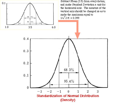
Thus standardized, 68.3% of the pupulation fall within -1 and 1 of the horizontal axis, and 95.4% fall within -2 and 2 (how can we obtain such values as 68.3? You will see in a minuite). Thus Standard Deviation (the unit of the horizontal axis) gives a good criterion for judging the extent of error contained in the data. And, in retrospect, you may think that Variance was so defined as to arrive at this nice result.
Incidentally, as Dr. Ishikawa aptly remarks, the notorious "hensa-chi偏差値" (deviation-value) used for judging your ability in schools (in Japan) is nothing but a transformed value from this standardized normal distribution; change 0 into 50 points, and change the unit 1 into 10 points, and the resulting value is the "hensa-chi". You can now see why "hensa-chi" 80 is rare!
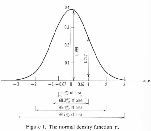
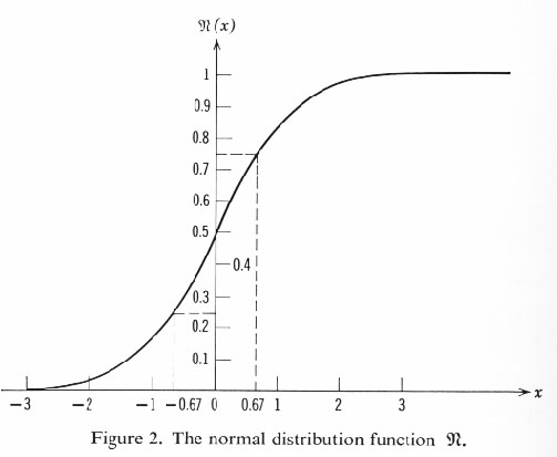
For a closer view of the standardized normal distribution (density and cumulative distribution), see the following figures reproduced (with a correction) from William Feller, An Introduction to Probability Theory and Its Applications, vol. 1, Wiley, 1968, p.178. Any standard textbook on statistics has a numerical table for the normal distribution, from which you can obtain probabilities of various sort. For example, assuming that the errors of measurement are governed by normal distribution, the probability that your measurement of a physical quantity falls within one standard diviation (from the true value, on both sides) is 0.683; and this value is obtained, formally by taking the integral of the corresponding middle part of the density function--but practically, by simple arithmetical calculations using the numerical table--, as is indicated in the Figure 1. Such technique as this is in the common arsenal of the sciences, and that's why Mayo uses the word "canonical".
Last modified Sept. 20, 2007. (c) Soshichi Uchii